不会吧不会吧,还有人学了三五遍还是不会动态规划算法?快戳 –>>
一、简单引入 · 斐波那契的例子
举个例子:计算斐波那契数列(1,1,2,3,5,…)的第n项
1. 暴力法(递归)
1 | int Fibonacci(int n) { |
但这是一个非常低效的办法。我们评判递归算法的性能一般采用递归树,那让我们画出上面算法的递归树:
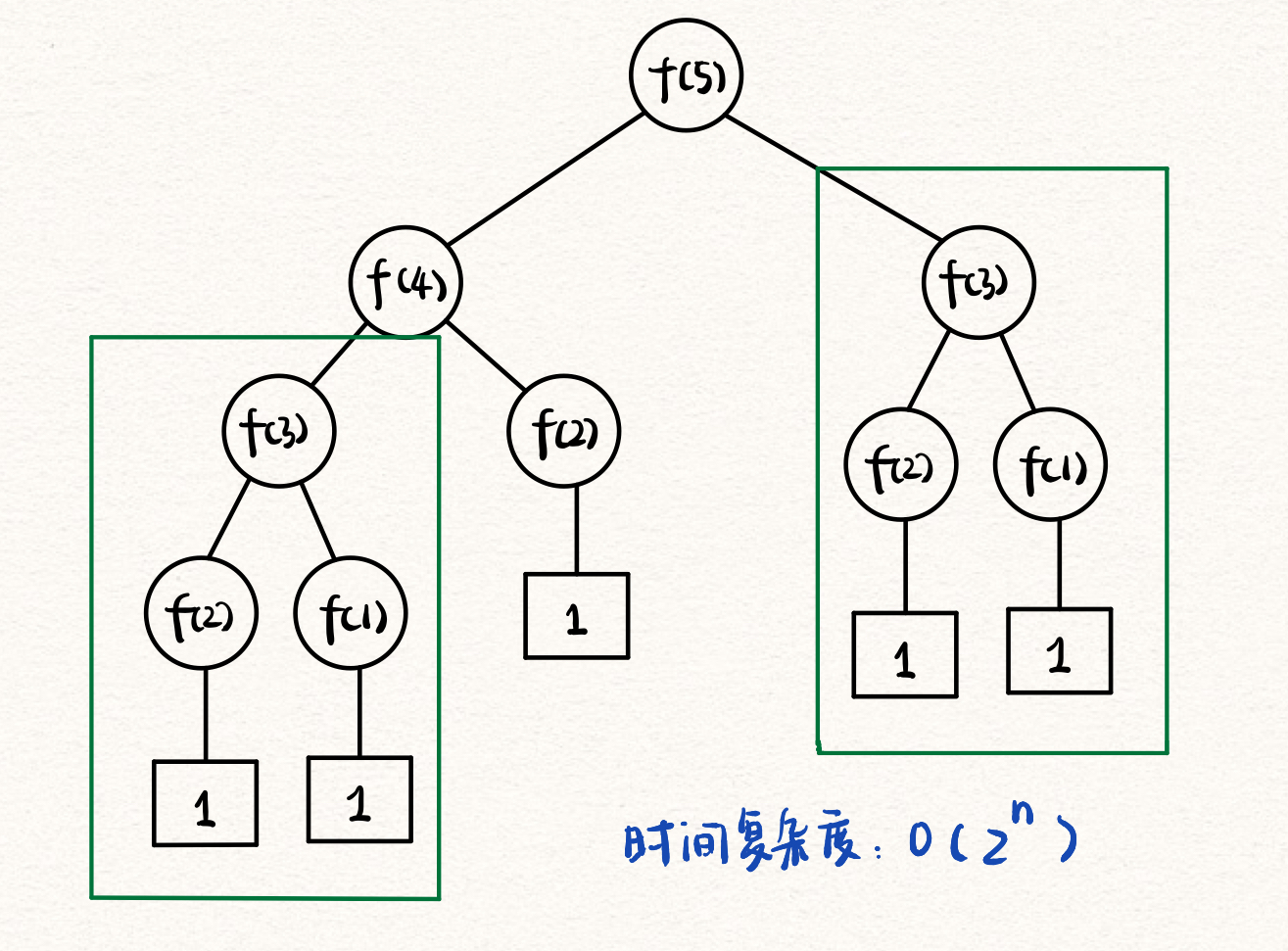
可以发现有很多的结点是在重复计算的,比如 f(3)。于是我们可以采用备忘录的方式(或者哈希字典)进行优化:
2. 备忘录方式
1 | int helper (vector<int>& memo, int n); |
执行结果对比:

可以发现,在数据量大的情况下(截图中为 f(40)),两种方法的效率有着质的差别。
在备忘录方法下,算法的时间复杂度又如何?以 f(40) 为例,算法只需要计算从 f(1) 到 f(40) ,所以 时间复杂度为 O(N) 。相比于暴力算法的时间复杂度 O($2^N$) 而言,这波空间换时间是超值了!
3. 动态规划
动态规划方法就是把“备忘录”独立出来,成为 DP_table,完成自底向上的计算。
1 | int Fibonacci3(int n) { |
其实斐波那契问题严格来说不算动态规划问题,毕竟没有涉及最优子问题。
二、第一个例子 · 凑零钱问题
有两种面值的纸币,2元、3元,每种纸币数量不限。
问:对于总额 amount,最少需要多少纸币才能凑出?若不能,返回 -1.
这给问题是一个典型的动态规划问题,因为他具有最优子结构。对于总额为 amount 时的最优方案,必然要求当总额为 amount - 2 和 amount - 3 时也是最优的,并且 changes[amount] = min(changes[amount - 2], changes[amount - 3]) + 1;。
此处 dp 数组 changes[amount] = n 的涵义为:当总额为 amount 时,最优解为 n ,即最少需要 n 张纸币才能凑出面额。
状态转移方程的数学表达式为:
$changes(amount) = \begin{cases} -1, & \text{当 $amount$ = 1} \\ 1, & \text{当 $amount$ = 2 或 3} \\ min{changes[amount - 2], changes[amount - 3]} + 1, & \text{当 $amount$ > 3} \end{cases}$
1 | int changes(int amount) { |
三、动态规划简介
动态规划(dynamic programming)和分治方法相似,都是通过组合子问题来解决原问题。
分治方法将问题划分为互不相交的子问题,递归地求解子问题,再将他们组合起来,求出原问题的解。与之相反,动态规划应用于问题重叠的情况,即不同的子问题具有公共的子子问题。动态规划对每个子子问题只求解一次,将结果保存在表格中,减少了重复计算的工作。—— 摘编自《算法导论》
一般我们可以从两个方面来判断一个问题能否用动态规划求解:
- 是否是最优解问题
- 能否分解为相互重叠的最优子问题
然后,
定义 dp 数组的具体含义
根据具体情况推导出状态转移方程,自底向上地进行解决。
四、Leetcode 动态规划 · 股票系列
1. 买股票的最佳时机(一)
https://leetcode-cn.com/problems/best-time-to-buy-and-sell-stock
给定一个数组,它的第 i 个元素是一支给定股票第 i 天的价格。
如果你最多只允许完成一笔交易(即买入和卖出一支股票一次),设计一个算法来计算你所能获取的最大利润。
注意:你不能在买入股票前卖出股票。
思路:股票问题的方法就是 动态规划,因为它包含了重叠子问题,即买卖股票的最佳时机是由之前买或不买的状态决定的,而之前买或不买又由更早的状态决定的。这题只需要做一次买卖,相对而言比较简单,可以不用动态规划,直接靠逻辑推理做出。我们将给出以上的两种办法。
逻辑推理法
首先,获得最大利润意味着我们希望在最小值处买入,在最大值处卖出。但需要明确,只有在买入以后才能卖出,可以卖出的前提是需要已经买入。所以,用更精炼的语言来说,我们希望在历史最低点买入,最高点卖出。因此,我们可以维护两个变量,分别为历史低价和最大差价,遍历每一个数据,不断更新历史低价和最大差价,最后输出最大差价。
1 | int maxProfit(vector<int>& prices) { |
动态规划法
我们用 dp 数组 maxprofit[i] 表示至 i 天的最大利润。那么我们可以列出状态转移方程:$maxprofit[i] = max\{maxprofit[i - 1], price[i] - minprice\}$。即至 i 天的最大利润只能是
$\begin{cases} 至 i- 1 天的最大利润:(第 i 天下跌了) \\ 当天价格 - 历史最低价:(第 i 天上涨了) \end{cases}$
1 | int maxProfit(vector<int>& prices) { |
2.买卖股票的最佳时机(二)
https://leetcode-cn.com/problems/best-time-to-buy-and-sell-stock-ii
给定一个数组,它的第 i 个元素是一支给定股票第 i 天的价格。
设计一个算法来计算你所能获取的最大利润。你可以尽可能地完成更多的交易(多次买卖一支股票)。
注意:你不能同时参与多笔交易(你必须在再次购买前出售掉之前的股票)。
同样这题较为简单,可以用逻辑推理和动态规划两种方法完成。
逻辑推理法
题目允许不限次数的交易,所以我们希望每次在价格开始上升的节点买入,在价格开始下降的节点卖出。但如果用变量来记录买入和卖出的状态会稍有繁琐,这里有一个本质上一样但在实现上更加美观简洁的理解:每当次日的价格较前日上涨,则累计增幅,最终累计的和就是题目要求的最大利润。
1 | class Solution { |
动态规划法
对于第 n - 1 天有两个状态:持有、未持有。对于持有状态,我们可以有两种操作:卖出、继续持有。对于未持有状态,我们可以有两种操作:保持不持有、买入。(此处 income[n] 为第 n 天最大收入)
第 n 天 $\begin{cases} 持有\begin{cases} (第n - 1天可能的情况)持有:income[n - 1] \\(第n - 1天可能的情况)不持有,在第 n 天买入:income[n - 1] - price[n] \end{cases} \\ 未持有\begin{cases} (第n - 1天可能的情况)不持有:income[n - 1] \\ (第n - 1天可能的情况)持有,在第 n 天卖出:income[n - 1] + price[n] \end{cases} \end{cases}$
我们定义状态 profit[i][] 的第二个维度为完成第 i 天的交易后是否持有股票。即 profit[i][0] 表示完成第 i 天的交易后不持有股票。
因此我们可以写出状态转移方程:
$\begin{cases} profit[i][0] = max\{profit[i - 1][0], profit[i - 1][1] + prices[i]\} \\profit[i][1] = max\{profit[i - 1][1], profit[i - 1][0] - prices[i]\} \end{cases}$
1 | int maxProfit(vector<int>& prices) { |
3.买卖股票的最佳时机(三)
https://leetcode-cn.com/problems/best-time-to-buy-and-sell-stock-iii/
给定一个数组,它的第 i 个元素是一支给定的股票在第 i 天的价格。
设计一个算法来计算你所能获取的最大利润。你最多可以完成 两笔 交易。
注意:你不能同时参与多笔交易(你必须在再次购买前出售掉之前的股票)。
思路:使用动态规划的办法。
二维dp表法
对于每一天有五个操作:$\begin{cases} state=0:没有操作 \\state=1:第一次买入 \\state=2:第一次卖出 \\state=3:第二次买入 \\state=4:第二次卖出 \end{cases}$
我们令 dp 表 profit[n][state] 表示第 n 天处于 state 状态时的最大利润。这五个状态和前一天的联系如下图所示:
$\begin{cases} state=0:没有操作 \\state=1:第一次持有\begin{cases} 当天买入:profit[n-1][0]-price[n] \\此前已经买入:price[n-1][1] \end{cases} \\state=2:第一次卖出\begin{cases} 当天卖出:profit[n-1][1]+price[n] \\此前已经卖出:profit[n-1][2] \end{cases} \\state=3:第二次买入\begin{cases} 当天买入:profit[n-1][2]-price[n] \\此前已经买入:price[n-1][3] \end{cases} \\state=4:第二次卖出\begin{cases} 当天卖出:profit[n-1][3]+price[n] \\此前已经卖出:profit[n-1][4] \end{cases} \end{cases}$
所以我们可以写出状态转移方程:
$\begin{cases} profit[0][0] = 0 \\profit[n][1] = max\{profit[n - 1][0] - price[n], profit[n - 1][1]\} \\profit[n][2] = max\{profit[n - 1][1] + price[n], profit[n - 1][2]\} \\profit[n][3] = max\{profit[n - 1][2] - price[n], profit[n - 1][3]\} \\profit[n][4] = max\{profit[n - 1][3] + price[n], profit[n - 1][4]\} \end{cases}$
1 | int maxProfit(vector<int>& prices) { |
一维dp表法
很显然,上一个办法使用了二维数组作为辅助空间,是一笔不小的空间开销。我们思考:能不能使用一维数组作为 dp 表呢?很容易发现在上个方法的状态转移方程中,第 i 天的值只和第 i - 1 天的相关,于是我们无需保存历史数据,只需要设置四个变量维护四种状态的最新值:
$\begin{cases} buy1:只进行过一次买操作 \\sell1:在一次买入后卖出 \\buy2:第二次买入 \\sell2:完成全部两笔操作 \end{cases}$
我们可以得到状态转移方程
$\begin{cases} buy1 = max\{buy1’, -price[i]\} \\sell1 = max\{sell1’,buy1’+price[i]\} \\buy2 = max\{buy2’, sell1’-price[i]\} \\sell2=max\{sell2’, buy2’+price[i]\} \end{cases}$
最后我们返回的值应该是 sell2 。因为首先最大利润一定是卖出状态,只能是 sell1 或者 sell2。如果最优解恰好是只完成一次交易即 sell1,也可以通过在最后一天买入并卖出转化成 sell2。
1 | int maxProfit(vector<int>& prices) { |
4.买卖股票的最佳时机(四)
https://leetcode-cn.com/problems/best-time-to-buy-and-sell-stock-iv/
给定一个整数数组 prices ,它的第 i 个元素 prices[i] 是一支给定的股票在第 i 天的价格。
设计一个算法来计算你所能获取的最大利润。你最多可以完成 k 笔交易。
注意:你不能同时参与多笔交易(你必须在再次购买前出售掉之前的股票)。
通过前三题的练习,不难想到可以根据题意列出 2*k + 1种状态,分别为:
$\begin{cases} state = 0:没有任何操作 \\state = 1:第一次买入\begin{cases}第n天买入:profit[n-1][0] - price[n] \\此前已经买入:profit[n-1][1] \end{cases} \\state = 2:第一次卖出\begin{cases}第n天卖出:profit[n-1][1] + price[n] \\此前已经卖出:profit[n-1][2] \end{cases} \\state = 3:第二次买入\begin{cases}第n天买入:profit[n-1][2] - price[n] \\此前已经买入:profit[n-1][3] \end{cases} \\state = 4:第二次卖出\begin{cases}第n天卖出:profit[n-1][3] + price[n] \\此前已经卖出:profit[n-1][4] \end{cases} \\…… \\state = 2k - 1:第k次买入\begin{cases}第n天买入:profit[n-1][2k-2] - price[n] \\此前已经买入:profit[n-1][2k-1] \end{cases} \\state = 2k:第k次卖出\begin{cases}第n天卖出:profit[n-1][2k-1] + price[n] \\此前已经卖出:profit[n-1][2k] \end{cases} \end{cases}$
很容易得到状态转移方程:
$\begin{cases} profit[n][2i-1] = max\{profit[n-1][2i-2] - price[n], profit[n-1][2i-1]\} \\profit[n][2i-2] = max\{profit[n-1][2i-1] + price[n], profit[n-1][2i-2]\} \end{cases}$
1 | int maxProfit(int k, vector<int>& prices) { |
5.最佳买卖股票时机含冷冻期
https://leetcode-cn.com/problems/best-time-to-buy-and-sell-stock-with-cooldown/
给定一个整数数组,其中第 i 个元素代表了第 i 天的股票价格 。
设计一个算法计算出最大利润。在满足以下约束条件下,你可以尽可能地完成更多的交易(多次买卖一支股票):
你不能同时参与多笔交易(你必须在再次购买前出售掉之前的股票)。
卖出股票后,你无法在第二天买入股票 (即冷冻期为 1 天)。
虽然题目很花哨,首先仍旧是确定状态:
对于第 n 天有两个状态:持有、未持有。对于持有状态,我们可以有两种操作:卖出、继续持有。对于未持有状态,我们可以有两种操作:保持不持有、买入。(此处 income[n] 为第 n 天最大收入)
第 n 天 $\begin{cases} 持有\begin{cases} 之前已经买入:income[n - 1] \\在第 n 天买入:income[n - 2] - price[n] \end{cases} \\ 未持有\begin{cases} 之前已经卖出:income[n - 1] \\在第 n 天卖出:income[n - 1] + price[n] \end{cases} \end{cases}$
上图中 n - 2 的含义是:考虑冷冻期,若要第 n 天进行买入操作,则第 n - 1 天必定不能进行卖出操作,income[n - 1] = income[n - 2];
我们定义状态 profit[i][] 的第二个维度为完成第 i 天的交易后是否持有股票。即 profit[i][0] 表示完成第 i 天的交易后不持有股票。
因此我们可以写出状态转移方程:
$\begin{cases} profit[i][0] = max\{profit[i - 1][0], profit[i - 2][1] + prices[i]\} \\profit[i][1] = max\{profit[i - 2][1], profit[i - 1][0] - prices[i]\} \end{cases}$
在下述代码中,笔者希望提醒各位读者重视初始值的设置以及边界的特殊处理。
1 | int maxProfit(vector<int>& prices) { |
6.买卖股票的最佳时机含手续费
https://leetcode-cn.com/problems/best-time-to-buy-and-sell-stock-with-transaction-fee/
给定一个整数数组 prices,其中第 i 个元素代表了第 i 天的股票价格 ;非负整数 fee 代表了交易股票的手续费用。
你可以无限次地完成交易,但是你每笔交易都需要付手续费。如果你已经购买了一个股票,在卖出它之前你就不能再继续购买股票了。
返回获得利润的最大值。
注意:这里的一笔交易指买入持有并卖出股票的整个过程,每笔交易你只需要为支付一次手续费
本题中,手续费是一件比较难处理的问题。该在算法的何时扣除手续费?不妨按三种情况思考:1.买入时一次性扣除;2.卖出时一次性扣除;3.买入时扣除一半,卖出时扣除一半。
笔者不才,难以用逻辑推理的方式选择方案,将上述三种情况分别做了实现。其中对买入时一次性扣除方案做了详细阐述。
买入时一次扣除
首先仍旧是确定状态:
对于第 n 天有两个状态:持有、未持有。对于持有状态,我们可以有两种操作:卖出、继续持有。对于未持有状态,我们可以有两种操作:保持不持有、买入。(此处 income[n] 为第 n 天最大收入)
第 n 天 $\begin{cases} 持有\begin{cases} 之前已经买入:income[n - 1] \\在第 n 天买入:income[n - 1] - price[n] - fee \end{cases} \\ 未持有\begin{cases} 之前已经卖出:income[n - 1] \\在第 n 天卖出:income[n - 1] + price[n] \end{cases} \end{cases}$
我们定义状态 profit[i][] 的第二个维度为完成第 i 天的交易后是否持有股票。即 profit[i][0] 表示完成第 i 天的交易后不持有股票。
因此我们可以写出状态转移方程:
$\begin{cases} profit[i][0] = max\{profit[i - 1][0], profit[i - 1][1] + prices[i]\} \\profit[i][1] = max\{profit[i - 1][1], profit[i - 1][0] - prices[i] - fee\} \end{cases}$
1 | int maxProfit(vector<int>& prices, int fee) { |
经过验证,结果正确。
卖出时一次性扣除
1 | int maxProfit(vector<int>& prices, int fee) { |
经过验证,结果正确。
买入时扣除一半,卖出时扣除一半
1 | int maxProfit(vector<int>& prices, int fee) { |
经过验证,结果正确。
这个方法存在一定的坑点:
通常我们在这题的题干下习惯将 fee 的类型设置为 int,若不加注意,在本题 fee / 2 时如产生小数将会对结果进行舍入,导致答案出错。例如:在高级编程语言整数除法的约定下,想必各位i读者对 3 / 2 = 1 应该不陌生。
若考虑到了坑点1所述的问题,但将 profit[][] 的类型设置为float,在较大整数下会出现问题:在32位机器下,有符号int类型是32位,即有效位数为31位;float类型小数部分为23位,对于超过24位的有符号Int类型转float,将会进行舍入。
类型 数符 阶码 尾数数值 总位数 偏置值(十进制) 偏置值(十进制) 短浮点数 1 8 23 32 127 7FH 长浮点数 1 11 52 64 1023 3FFH 临时浮点数 1 15 64 80 16383 3FFFH 显而易见,如使用 double 类型则可以满足有符号 int 类型的位数需求。
以上“位数”均为机器数位数)
五、总结
如果遇到的问题是求最优解问题,并且存在重叠子问题,则可以考虑使用动态规划算法求解。
是用动态规划方法,重中之重是定义状态,写出状态转移转移方程
至此,便可以开始着手编写程序代码。
在此笔者尤其想提醒各位读者:不要轻视 dp 数组初始值的设定和对于给定参数边界值的处理!
写在最后:本文是笔者在经历了几次动态规划问题的学习之后,参考部分资料并结合自己的理解,整理出的一篇动态规划入门学习文章。对于第四章所举的例子,目的为利用相近情境的题目提升趣味性,可能覆盖的方法与技巧不够全面,后续可能会进行修改。如有疏漏,欢迎读者在评论区指正!
参考资料:leetcode 平台(https://leetcode-cn.com/),书籍《labuladong的算法小抄》《算法导论(第三版)》《算法笔记》,以及网络各类资料。